This post is part 1 of the "Empirical Bayes" series:
- Shrinkage and Empirical Bayes to improve inference
- Empirical Bayes with regression
- Derivations and Conjugate Priors (average ratings)
- Derivations and Conjugate Priors (proportions)
Shrinkage and Empirical Bayes to improve inference
There is a common problem when ranking items: if we just average the observations, fluctuations tend to make the very best (and very worst) items be those with very few observations. Consider the following three examples:
- We are trying to measure the batters with the best hit rate. A rookie that has hit 2 balls out of 2 at-bats would have a hit rate of 1.0, handily beating Barry Bond's career hit rate of 0.306. To get hit rates over 0.300 is rare in major league baseball, so we are confident that the rookie's hit rate isn't 1.000.
- When looking at kidney cancer incidence rates per county. It is a relatively rare disease, with the lowest rate being 6.6 per 100k in Garfield County (4 out of 60000), and a highest rate of 41.1 per 100k in Cass County (7 out of 17000). Having just one fewer person diagnosed with kidney cancer in Cass County would drop the rate to 35.2 per 100k. There are 63 counties that where the 95% confidence interval in the rate exceeds 41.1 per 100k.
- We are trying to measure the rating of a book. A book with two 5 star ratings probably isn't better than a book with ten thousand ratings that average to 4.85.
In each of these cases, just measuring the average over all items isn't useful. We want to know what the hit rate is of an individual player, the counties that have abnormally high kidney cancer rates, or the our best estimate of the rating of a particular book. One way of approaching this would be to have a cutoff and refuse to make any inference before we had "enough" data.
Empirical Bayes approaches this problem differently. We use the entire population (that is, all players, all counties, or all books) to estimate what a "typical" result looks like. If we had no batting data, for example, we can still say based on all major league players that a given player is likely to have a hit rate between 0.2 and 0.3. We use this as the prior. This is the empirical part. As we collect more and more data, we use Bayes's rule to update our prior. When we have only a little bit of data on a player, county, or book, the prior is important for keeping our estimates grounded. As we get more data, the initial prior becomes less and less important, which matches our intuition that the large fluctuations needed to significantly bias large datasets are rare.
This general technique of moving the observed data toward the mean is also called "shrinkage" (although maybe "regression", as in "regression to the mean" would be a better name).
David Robinson has already given an excellent treatment of empirical Bayes in the context of baseball statistics on his blog, variance explained. We will look at the two other examples above in this blog post:
- We will look at the kidney cancer rates per county. This example has been discussed in "Thinking Fast and Slow" by Daniel Kahneman. The data set is available here
- We will look at the ratings of boardgames given at boardgamegeek. This problem was inspired by the 538 article "Worst board game ever invented". In this case, the ratings were not shrunk, so games with fewer reviews typically showed more variance. The data set for this problem is available here.
By using these two examples, we can show how to apply the empirical Bayes's technique of "shrinking" (or regressing) our observed values toward the mean when estimating a proportion (kidney cancer rates) as well as a continuous variable (board game ratings).
NOTES
- This notebook is mostly written to expose the reader to the idea of shrinkage, and be able to apply it quickly. For that reason, code is included but the derivations are not. The derivations of the formula are available in a more detailed article.
- Data and the notebooks are available here.
Case study 1: Shrinking proportions with kidney cancer data
Let's start by getting an overall view of the kidney cancer rates. Our first attempt might be to simply make a histogram of the kidney cancer rate.
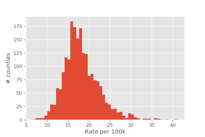
It is relatively simple to identify the lowest and highest observed rates directly from the histogram. But by displaying this data as a histogram, we haven't displayed the sample size of each county, so it isn't clear how reliable each of the individual measurements are. The story looks very different once we add population size as an axis. The overall average rate (as measured over the entire US) is shown as a dashed line.
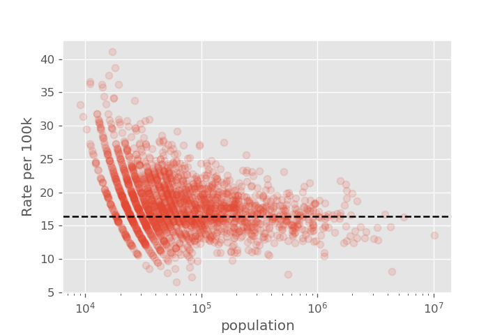
We see that there is a lot more variation in cancer rates for the counties with small populations, with the variation getting smaller as we go to larger counties. This is the type of behavior we expect from statistical fluctuations!
Overview of method
We are going to assume that each county \(i\) is described by a kidney cancer rate, \(p_i\). The \(p_i\) are randomly distributed according to the histogram of kidney cancer rates we plotted earlier. That is, if we had a probability distribution that matched the shape of this histogram, we could tell how likely it was that a particular cancer rate \(p_i\) was observed.
It is convenient if we can model this process using a \(\beta\)-distribution. The \(\beta\) distribution is described by two parameters, s0 and f0, which we can think of as "banked" successes and failures. If we observe s_i actual sick people in a county, and f_i healthy people in the county, then the naive calculation for the rate people are getting sick is
The empirical Bayes method would adjust this estimate to
One way of thinking about this result is that we are pretending that we have s0 sick people and f0 healthy people that are not actually part of our population. When calculating the rate, we still look at the ratio of sick people to the total, but we also include the (s0 + f0) "imaginary people" we are using to represent the rest of the population.
Step 1: Use population data to get prior
Since we are modeling a binomial process (in each county, an individual either does or does not get sick), it is convenient if we can model this distribution with a \(\beta\)-distribution. One way of doing this is called the "method of moments", where we find s0 and f0 to make the mean and variance of the beta distribution match the mean and variance of our data. The formula are
Instead of trying to match mean and variance, we can use the built-in fit method for finding the parameters:
from scipy.stats import beta
s0, f0, *extra_params = beta.fit(incidence['Rate_per_100k']/1e5, floc=0., fscale=1.)
The values for these parameters are \(s_0=19.4\) and \(f_0=106389\). That is, for every county we imagine there are an additional 19 sick people, and an additional 106389 healthy people.
We can visualize how well this plot did with the following code, using beta.pdf with our parameters to plot our fitted beta distribution.
plt.figure(dpi=130)
X = np.linspace(0, 0.001, 200)
plt.plot(X, beta.pdf(X, a=s0, b=f0, loc=0, scale=1), label='Beta dist')
plt.hist(incidence['Rate_per_100k']/1e5, bins=50, normed=True, label='data')
plt.xlim(0,5e-4)
plt.title('Best fit beta distribution')
plt.legend()
plt.xlabel('Prob of Kidney Disease')
plt.ylabel('PDF');
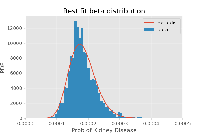
The fit isn't terrible, but a slightly smaller lump around 0.00023 suggests we might have two different mixed beta distributions. We could improve the fit slightly by modeling our prior as two beta distributions, but this would complicate our shrinkage. We still find a reasonable fit with s0 and f0.
The downside to using the best-fit method is that the average rate is shrunk toward the average of the beta distribution, not the average of the data. We can find the average of the beta distribution directly from the parameters s0 and f0:
By comparison, the average from the data is 16.1 per 100k.
Step 2: Use prior to "shrink" estimates to population values
Our dataframe incidence has the following columns:
'average_annual_count': the number of people in the county that we found the disease.'population': the population of the people in the country.
To get our empirical Bayes estimate needs us to add s0 to the number of detected cases, and s0 + f0 to the population. Recalling that we are reporting rates per 1e5 people, the calculation for the corrected column is simple:
incidence['shrinkage'] = 1e5*(incidence['average_annual_count'] + s0)/(incidence['population'] + s0 + f0)
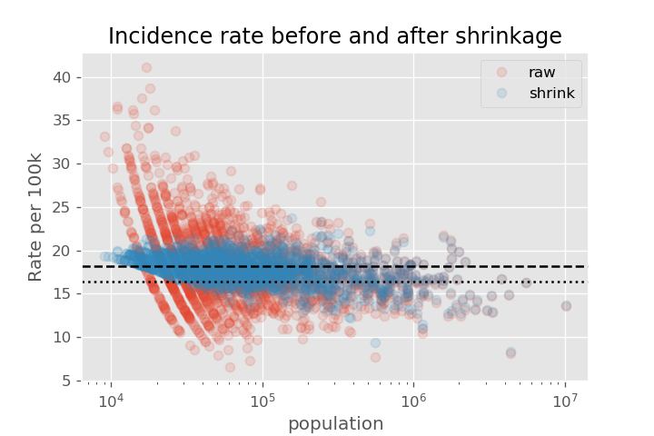
Let's compare what the rates looked like before and after the shrinkage. We recreate the plot of cancer rate vs population. Note the shrinkage effect is much larger for the smaller populations. We also show the dashed line that we shrink toward (approx 18 per 100k), as well as the average of the actual data as the dotted line (approx 16 per 100k).
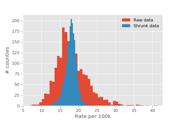
Now that we have our best estimate based on the sample size, we can plot a histogram of the adjusted rate.
Case study 2: Shrinking continuous data with board game ratings
This time, we will look at correcting the average of a continuous variable, instead of a rate. The website BoardGameGeek collects user and critic ratings of many different board games. If we look at the average rating of each game with more than 30 ratings, we get the following histogram
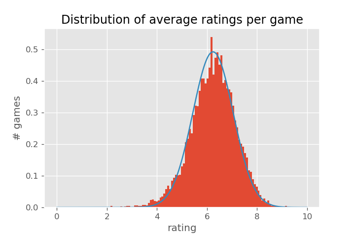
(Games with very few ratings tend to concentrate around integer and half-integer ratings, which puts visual "spikes" in the histogram.)
After the previous discussion, might be wondering how confident we are in the extreme ends of the distribution. We would expect that the games with few reviews would have an easier time getting a very high or very low review score. Let's check this intuition by plotting review score against the number of reviews.
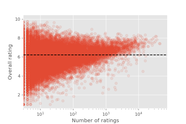
Once again we see the "triangle shape" indicating that the tails of the distribution are dominated by the data we are least confident in. Since we are modeling sample means (i.e. the average rating given to a board game by the users), the central limit theorem tells us that the sample means will be normally distributed around the true mean.
We also note that there is some bias in the results: instead of the distribution just narrowing down as the game becomes more popular, there is a fairly distinct upward rise in average ratings as the game becomes more popular. We will address this in a more detailed article on empirical Bayes with regression; in this article we will just take a naive approach.
Our distribution above suggests we won't go too far wrong by taking the distribution actual game scores to be normally distributed. Yes, the logic here isn't completely airtight -- we are using the distribution of sample means to infer the distribution of actual means -- but this is the "empirical" part of empirical Bayes!
Some notation
Before breaking down the methodology, we should introduce some notation. First we have some global parameters, which describe the distribution of game ratings:
| Parameter | Meaning |
|---|---|
| \(\mu\) | The average score of all board games (i.e. the average in the histogram above) |
| \(\tau^2\) | The variance in ratings of all board games (i.e. the variance in the histogram above) |
We also have parameters on a per game basis. Since the dataframe games has one row per game, with summary statistics, and not the individual reviews, we include the column name used in the code
| Parameter | Meaning | Column name |
|---|---|---|
| \(\theta_i\) | The underlying (unknown) rating of the game \(i\) | (not available) |
| \(\bar{x}_i\) | The average measured rating of game \(i\) (i.e. the naive average rating per game) | 'average_rating' |
| \(\sigma_i^2\) | The variance in the ratings of game \(i\) | 'rating_stddev' |
| \(n_i\) | The number of reviews for game \(i\) | 'users_rated' |
| \(\epsilon_i^2\) | The standard error in the rating of game \(i\), which is \(\sigma_i^2/n_i\) | (calculated) |
Step 1: Calculate the population parameters
We can estimate the population mean and variance directly from the series 'average_rating'. In this example, I did it the lazy way:
MIN_REVIEWS = 30
subset_mask = (games['average_rating'] > MIN_REVIEW)
rating_masked = games.loc[subset_mask, 'average_rating']

# This is our population mean
mu = rating_masked.mean()
# This is our population variance
tau2 = rating_masked.var()
The less lazy way of doing it would be to take a weighted average and a pooled variance, so that games with more reviews influenced the population mean more. The above method is a nice to get a quick-and-dirty estimate.
Step 2: Get the standard error
This uses the central limit theorem (CLT) to estimate the error we have in the estimate of the mean on a per game basis. The CLT tells us that the sample mean (i.e. our measurement ) will be drawn from a normal distribution around the true (unobserved) mean \(\theta_i\) and variance \(\epsilon_i^2 = \sigma_i^2 / n_i\). In code:
# These are our epsilon_i^2
games['std_var'] = games['rating_stddev']**2/games['users_rated']
Step 3: Calculate the interpolation factor
For each game, we have to weigh how much of the rating comes from the observed rating for that game, and how much comes from the overall population. The following factor, \(B_i\), does this for us:
If we have a lot of ratings for a game, and the variance in the ratings for that game are low, we have \(\epsilon_i^2 \ll \tau^2\), so \(B_i \approx 1\). When \(B_i\) is close to 1, we expect most of the contribution to come from the ratings on the game.
On the other hand, if we have relatively little information on the game, \(\epsilon_i^2 \gg \tau^2\), so \(B_i \approx 0\). This is where we would expect the global average to be important.
We will see in step 4 that this intuition holds. In our derivation article we will show where this formula comes from, but at the moment it is enough to gain an intuition of what \(B_i\) close to its two extremes means.
To calculate this factor in code is simple:
games['interpolation'] = tau2 / (tau2 + games['std_var'])
Step 4: Regress/Shrink the measured value
We can use the interpolation factor in the previous step with the following formula:
In code, this is
games['shrunk_rating'] = games['interpolation']*games['average_rating'] + (1-games['interpolation'])*mu
That's it -- we are done!
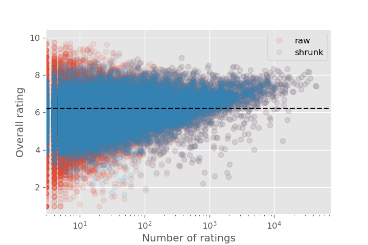
Here is the plot of the ratings vs population size, showing the distributions both before and after applying shrinkage.
Summary
We can do better than looking at an overall average rate or rating, especially when dealing with small sample sizes. We know that it is easier to move an average when there are only a small number of measurements; if we know what the overall distribution of measurements should look like we can correct the small samples. By allowing results to "shrink" (or "regress") to the mean, you make the results for your "best-of" and "worst-of" lists much more stable.
The techniques in this article are most useful for analytics tasks, where you are being asked to generate reports or make insights based on what has already happened. If you are building a machine learning model on average rates, such as trying to predict the factors that influence the cancer rate of a county, you have a couple of different approaches:
- Use the techniques in this article, and fit to the "shrunk" estimates
- Use the actual measured averages, but introduce a weighting factor so that measurements averaged over fewer observations carry less weight.
This is an important point that can hang up many beginning data scientists, as discussed in Cameron Pilon on his PyData talk "Mistakes I've Made".
This article showed two different techniques for empirical Bayes, one for correcting rates and the other for correcting regression (of averages).
Correcting rates
- Model the distribution of rates in your data using the beta-distribution. Call these parameters \(s_0\) and \(f_0\).
- For each sample (e.g. county) with \(s\) "successes" and \(f\) "failures", shrink the rate using the following technique:
$$\text{rate} = \frac{s + s_0}{(s + f) + (s_0 + f_0)}$$
Correcting averages
- Model the distribution of averages in your data using the normal distribution. Use the mean \(\mu\) and variance \(\tau^2\) of this distribution.
- For each sample (e.g. board game) with an average of \(N_i\) reviews and variance in measurements, \(\sigma_i^2\), the central limit theorem tells us that our measurement of the mean will have a variance \(\sigma_i^2/N_i\).
- For each sample, define
$$B_i = \frac{\tau^2}{\tau^2 + (\sigma^2_i/N_i)}$$Note that when \(B_i\approx 1\), we have \(\sigma^2_i/N_i \ll \tau^2\), meaning that we are much more certain about this measurement than the overall variation in the population, so we expect our measurement to dominate. When \(B_i \approx 0\), we have \(\sigma^2_i/N_i \gg \tau^2\), so we expect fluctuations from this single sample to be much bigger than the population standard deviation (so shrinkage will dominate).
- The "shrunk" estimate for sample \(i\) is
$$\text{rating} = B_i \bar{x}_i + (1 - B_i) \mu$$where \(\bar{x}_i\) is the (raw) measured rating over the \(N_i\) measurements.
Other resources
This article hasn't focused on the mathematical derivations, if you are interested a follow up article is here. Another nice resource on empirical Bayes is David Robinson's blog, Variance Explained. A project on when using empirical Bayes it is useful (and when it isn't) in epidemiological studies is available here.
Finally, the data cleaning and notebooks for this project are available here.